
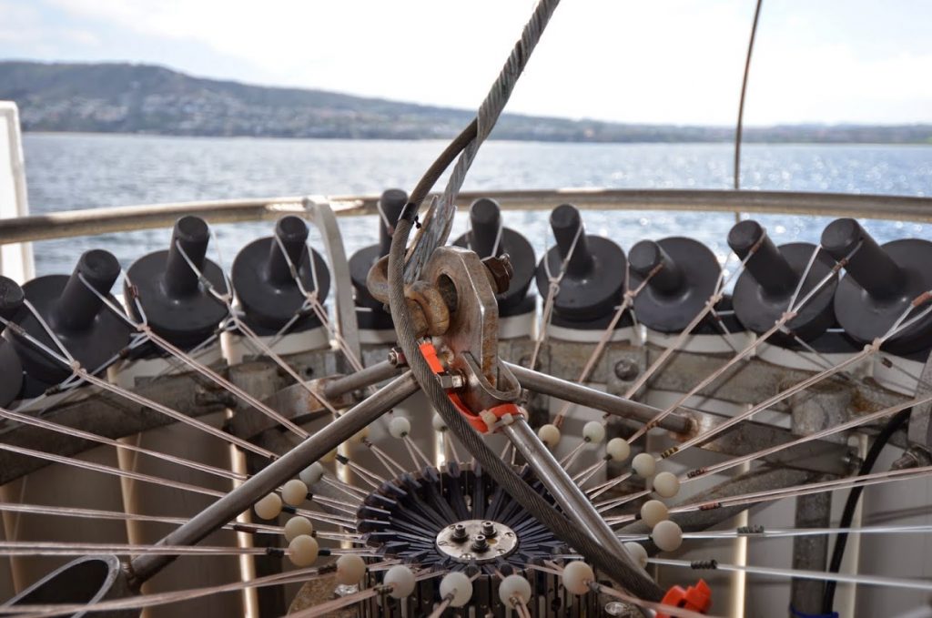
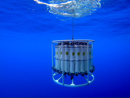
Bottle Sampling
The Sea-Bird Electronic Carousel Water Sampler (SBE 32) uses an electromagnetically activated lanyard release system to close 24 ten-liter plastic (PVC) bottles equipped with epoxy-coated springs and Viton O-rings.
Each cast typically samples ~20 depths to a maximum sampling depth of 515 meters, bottom depth permitting. Two deeper CTD casts are performed at the Santa Monica Basin (770m) and Santa Barbara Basin (570m).
Some stations have multiple bottles tripped at the same depth to provide additional water for ancillary measurements.
The sampling depths are based on the chlorophyll maximum and mixed layer depths profiled during the CTD downcast. Using the CTD down cast fluorometer profile to determine the chlorophyll max depth, 10m bottle spacing shifts up or down. Distributing the higher resolution 10m bottle spacing around the chl max.
Salinity, oxygen, and nutrient analyses are done at-sea for all depths sampled. Chlorophyll-a and phaeopigments are also analyzed at-sea on samples from the upper 200 meters, bottom depth permitting.
Standard CalCOFI Bottle Measurements
LTER Bottle Measurements
- POC & PON
- TOC & TN
- Nano-Microplankton
- Picophytoplankton
- Size Fractionation
- Phyto-Pigments
Particulate Organic Carbon & Nitrogen
CCE LTER measures particulate organic carbon (POC) and nitrogen (PON) by high-temperature combustion. Samples analyzed within the California Current Ecosystem constrain the mean C:N ratio of small particulates and by difference relative to measured living biomass, the biomass of suspended detritus.
Complete methods for POC and PON determination can be found here
Principle
For the analysis of particulate organic carbon and nitrogen (POC/PON) 4 liters of seawater are filtered on glassfiber filters and stored at -20°C for analysis ashore. Ashore samples are acidified, dried and analyzed by high-temperature combustion (1000°C) on an ECS 4010 CHNSO Analyzer. The sample and tin capsule react with oxygen and combust at 1000°C. The sample is broken down thus converting organic carbon to CO2 and reducing nitrogen oxides to N2 gas. Both gases are measured by thermal conductivity.
Sampling
POC/PON samples are collected for 66 CalCOFI stations and 9 SCCOOS stations located in the CCE. Three to eight depths are sampled. POC/PN samples are collected in 0.5, 1.04 or 2.2 Liter, brown polypropylene bottles. Smaller volumes are collected when high chlorophyll concentrations are measured from the CTD fluorometer. High concentrations are typically measured around the coastal stations. 3.2. Samples are filtered on precombusted Whatman GF/F 25mm under low vacuum pressure (40 mm Hg). 3.3. Filter is removed, folded in half with the particulate part inside the fold and wrapped in precombusted aluminum foil. 3.4. Samples are stored in Liquid Nitrogen and transferred post cruise to a -20°C freezer until processed.
Dissolved Organic Carbon & Total Nitrogen Sampling
CCE LTER analyzes and determines total organic carbon (TOC) and total nitrogen (TN) in sea water, expressed as micromoles of carbon (nitrogen) per liter of sea water. TOC (<200 µmol·L-1) includes both dissolved and particulate organic carbon (DOC and POC, respectively). TN (<50 µmol·L-1) includes particulate and dissolved organic nitrogen as well as dissolved inorganic nitrogen species. The instruments employed are from the Aluwihare Laboratory at the Scripps Institution of Oceanography, and whenever possible, protocols closely follow those used by Jonathan Sharp (U. of Delaware), Craig Carlson (U. of California, Santa Barbara) and Dennis Hansell (RMSAS). SIO has the Shimadzu TOC-VSN, normal sensitivity, with TN unit.
Complete methods for TOC and TN determination can be found here
Principle
An acidified seawater sample (< pH 3) is sparged with CO2 free-air to remove inorganic carbon. The water is then injected onto a combustion column packed with platinum-coated alumina beads held at 680°C. Non-purgeable organic carbon (NPOC) compounds are combusted and converted to CO2, which is detected by a nondispersive infrared detector (NDIR). Non-purgeable nitrogen compounds (which includes organic and inorganic nitrogen species) are combusted and converted to NO, which when mixed with ozone chemiluminesces for detection by a photomultiplier.
Sampling
All samples collected on CalCOFI and LTER cruises are TOC and TN samples. That is, no filtering of the sample is done to remove particulates. Filtering is time-intensive and filtration, especially by untrained personnel, can introduce significant contamination. So, to maximize efficiency and minimize sample handling, the filtration step common to DOC and TDN is omitted. In open ocean waters particulate organic carbon concentrations are a small fraction of the total organic carbon and does not pose too many problems. Here subtracting POC from TOC is likely to provide an accurate estimate of DOC because particles are typically small and homogeneously distributed in the sample. In coastal waters, and at stations where relatively high chlorophyll concentrations are present, the TOC measurement cannot be easily converted to DOC by subtracting POC values. Experience has shown that particles in these regions are large and inhomogeneously distributed. Therefore, samples collected in this study are reported as TOC and TN.
Sampling Depths
Water samples are taken directly from the CTD-Rosette.
SCCOOS stations: Full profiles are taken (4-5 vials per station).
Line 93.3 has mostly “normal” stations, which means samples are drawn from the surface Niskin, the deep Niskin, and three LTER depths (5 vials in all).
- At 93.3 55 and 93.3 90 samples are drawn from Niskins triggered at 13 depths between 0 and 170 m, and 230 m, 320 m and the deepest Niskin (16 vials).
Line 90.0 has a mix of normal, LTER cardinal, and full profile stations.
- Normal stations (28, 30, 35, 45, 60, 80, and 100) sample surface, deep, 3 LTER depths, 140/145m, and 320 m.
- Cardinal stations (37, 70, 90 and 120) sample surface, deep, 6 LTER depths, 140/145m, 230 m and 320 m.
- Full profiles are collected at station 100 and 53 (20-24 vials).
Line 86.7 is primarily sampled at the surface, deepest, 3 LTER depths, 140/145m and 320m.
- A full profile is taken at the Santa Monica Basin station (86.7 40).
- 16 samples are collected at 60 and 100, which include deepest, 230 m, 320 m and 13 samples between 0-170 m.
Line 83.3 is similar to 93.3. Most stations are sampled at the surface, deepest bottle, and 3 LTER depths.
- Stations 90 and 70 are sampled at the deepest depth, 230 m, 320 m and 13 depths between 0-170 m.
- A full profile is collected at 81.7 46.9 (Santa Barbara Basin).
Line 80.0 is similar to Line 90.0.
- Stations 51, 60, 90 are sampled at the surface, deepest bottle, 3 LTER depths, 140/145 m and 320 m.
- Full profiles are taken at station 55 and 100.
- Remaining stations are cardinal stations which include surface, deepest bottle, 6 LTER depths, 140/145 m and 320 m.
Line 76.7 is sampled primarily at the surface, deepest bottle, and 3 LTER depths.
- Stations 55, 70 and 90 are sampled at the deepest bottle, 230 m, 320 m and 13 depths between 0-170 m.
Nano-Microplankton Abundance & Biomass
CCE-LTER asseses the microbial community assemblages of the California Current ecosystem (CCE) for abundance and biomass using high-throughput digital epifluorescence microscopy. Samples to estimate the nano- and microplankton (0.2-2.0-µm and 2.0-20-µm size, respectively) are collected, preserved, stained, and filtered onto a membrane filter and mounted on a glass microscope slide in the field. Slides are then frozen at -80°C for subsequent imaging and analysis in the laboratory onshore.
Complete methods for microbial community assemblage assessment can be found here
Principle
Microscopical assessment of nano- and microplankton: Aliquots of 50- and 500-ml are collected for analyses of nano- and microplankton by digitally enhanced epifluorescence microscopy. Samples for nano- and microplankton abundance and biomass are preserved and then stained. Preserved samples are allowed to fix prior to gentle filtration onto 0.8-µm (nano) or 8.0-µm (micro) pore size filters. Filters are mounted onto glass slides with immersion oil and cover slip. Slides are stored at -80°C for analysis back on shore.
Sampling
Nano- and microplankton are sampled from 3 to 8 depths for each of the 66 CalCOFI stations located in the CCE. Seawater from the Niskin bottle is collected into a 600-ml sample bottle. When sampling, make sure the flow from the valves is low since no sample tubing is used.
Picophytoplankton & Prokaryotes
CCE-LTER samples picophytoplankton populations and non-pigmented prokaryotes within the California Current Ecosystem (CCE) are fixed in the field by the addition of paraformaldehyde and, in the laboratory, stained with Hoechst 33342 (a DNA specific dye). The cells are enumerated by an Altra flow cytometer and converted to biomass estimates.
Complete methods for picoplankton and bacteria abundance and biomass determination can be found here
Principle
Flow cytometric analyses of picoplankton populations (Prochlorococcus, Synechococcus, P-Euk and H-Bact) are preserved with paraformaldehyde, frozen in liquid nitrogen, and stored at -80°C. Prior to analysis, batches of thawed samples are stained to increase the precision of bacterial counts, relative to epifluorescence microscopy. Aliquots are analyzed using a Beckman-Coulter EPICS Altra flow cytometer with a Harvard Apparatus syringe pump for volumetric sample delivery.
Sampling
Picoplankton and bacteria are sampled from 3 to 8 depths for each of the 66 CalCOFI stations located in the CCE. Seawater from the Niskin bottle is collected into a 600-ml sample bottle. When sampling, make sure the flow from the valves is low since no sample tubing is used. A 2-ml subsample is drawn from the sample bottle and placed into a properly labeled 2-ml cryovial, and 100 µl of prefiltered 10% paraformaldehyde is added (0.5% final v/v sample concentration). Samples are left out for 10 min and then stored in liquid nitrogen. At the shore-based laboratory, the samples are stored at -80°C. Samples are shipped overnight on dry ice to SOEST Flow Cytometry Facility, University of Hawaii at Manoa for flow cytometry analysis.
Size Fractionation
CCE-LTER determines the size distribution of total chlorophyll a by filtering water though filters of differing pore sizes, extracting these in acetone and analyzing fluorometrically. Using size fractionation of chlorophyll a and taxon-specific pigments (chlorophylls and carotenoids) from HPLC analysis, the samples analyzed within the California Current Ecosystem are used to develop a metric for phytoplankton community structure that can be used to monitor its state and changes thereof over time.
Complete methods for chlorophyll-a size fractionation can be found here
Principle
For the size fractionation of chlorophyll a, a 10 meter depth sample of seawater is collected, filtered in parallel through filters with five different pore sizes (GF/F filters, 1 µm, 3 µm and 8 µm, and 20 µm pore sizes), and these are extracted in 90% acetone for 24 hours in the dark at -20°C for standard fluorometric analysis. Each size treatment has 3 replicates.
Sampling
Water for size fractionation of chlorophyll a is sampled from a 10m depth on Line 83 and 87 with scattered inshore stations within the CalCOFI and SCCOOS stations located in the CCE. A seawater sample (about 4.5 – 5 liters) is collected from the Niskin bottle in a 10 liter carboy.
Taxon-Specific Phyto-Pigments
CCE-LTER uses a high-performance liquid chromatographic (HPLC) method with a reverse phase C8 column to measure concentrations of chlorophylls and carotenoids in samples of particulate matter from the California Current Ecosystem (CCE). Concentrations of chlorophyll a are used as a proxy for phytoplankton biomass and concentrations of other taxon-specific pigments are used to determine contributions of phytoplankton taxa to total phytoplankton biomass.
Complete methods for taxon-specific phyto-pigments determination can be found here
Principle
Chlorophylls and carotenoids are extracted from samples collected on CalCOFI (California Cooperative Oceanic Fisheries Investigations) cruises with acetone. The extracts are analyzed on an Agilent 1100 series HPLC with a thermostatted autosampler derived from the method described in Zapata et al. (2000).
Sampling
HPLC samples are collected at CalCOFI and SCCOOS (Southern California Coastal Observing System) stations located within the CCE. Samples are collected from three to eight different depths in the photic zone. Samples are drawn from the niskin bottles using 0.5, 1.04 or 2.2 liter brown polypropylene bottles, depending on the chlorophyll concentration measured by the fluorometer on the CTD. For the higher chlorophyll values, typically the coastal stations, less water is sampled. Samples (0.5, 1.04, or 2.2 L) are filtered onto 25 mm GF/F filters (Whatman) under a low vacuum pressure (≤ 40 mm Hg). 2.4. Once the sample has finished filtering, the filter is carefully folded in half, and blotted on a paper towel to remove excess water. The folded filter is placed in a labeled 2 ml cryovial and stored in liquid nitrogen for analysis ashore.
- Salinity
- Dissolved Oxygen
- Nutrient
- Chlorophyll-a
- Primary Productivity
Salinity Sampling
On each station, seawater salinity samples of ~225 mL are drawn from all CTD-rosette bottles closed during the cast. A Guildline Instruments Portasal™ Salinometer (8410A) measures the seawater sample conductivity precisely, comparing it to a reference seawater standard. From these comparisons, salinities are calculated and logged using Windows-PC based software that averages data that meet replicate criteria. Concurrent with the water sampling, a Sea-Bird Electronics CTD equipped with dual conductivity meters profiles in situ data. Data processing software is then used to compare the bottle salts to in situ CTD measurements. These are used to confirm bottle closures at target depths, monitor CTD sensor performance, and helps select the best salinity data for future comparison and publication.
Complete methods for salinity determination can be found here
Sample Bottles
Salinity bottles are collected in ~250 ml borosilicate KIMAX-35 bottles. These square cross-sectioned bottles have screw tops with separate plastic thimbles to prevent leakage and evaporation. Numbered, stackable divider boxes hold 24 numbered bottles to match the 24 Niskins on the rosette. Bottles are left filled with previously unused sample water to limit salt crystallization and to pre-leech silicate from the glass.
Sample Collection
Numbered salt bottles are matched to the corresponding Niskin bottles and filled to the shoulder after three ~40 ml rinses. The last fill is done without interruption until overflowing; then ~10 ml is poured out over the thimble and the bottle is stoppered and capped. Samples are left to equilibrate to room temperature for at least 8 hours prior to analysis. Before being placed on the salinometer, samples are: gently inverted 3 times to remove any possible stratification; after being uncapped, seawater trapped around and under the thimble is ‘wicked’ away using a Kimwipe; if the thimble falls off before the removal of trapped seawater or ‘champagnes’ off the sample bottle, ~10-20 ml of the sample is dumped into a collection bucket.
Guildline Portasal™ Salinometer (8410A)
Guildline Portasal Salinometer model 8410A is used to make the precise conductivity comparisons between the water samples and reference water standards. Two of these instruments are taken on each cruise. Guildline specifications state an accuracy of ±0.003 PSU (same set point temperature as standardization and within -2°C and +4°C of ambient), and a precision of 0.0003 PSU.
Dissolved Oxygen Sampling
The amount of dissolved oxygen in seawater is measured using the Carpenter modification of the Winkler method. Carpenters modification (1965) was designed to increase the accuracy of the original method devised by Winkler in 1889. Using Carpenters modification, the significant loss of iodine is reduced and air oxidation of iodide is minimized. Rather than using the visible color of the iodine-starch complex as an indicator of the titration end-point, we use an automated titrator that measures the absorption of ultraviolet light by the tri-iodide ion, which is centered at a wavelength of 350 nm.
Complete methods for dissolved oxygen determination can be found here
Principle
Manganous chloride solution is added to a known quantity of seawater and is immediately followed by the addition of sodium hydroxide iodide solution. Manganous hydroxide is oxidized by the dissolved oxygen in the seawater sample and precipitates forming hydrated tetravalent oxides of manganese.
Mn+2 + 2OH- ———————————————-> Mn(OH)2 (solid)
2Mn(OH)2 + O2 ——————————————–> 2MnO(OH)2 (solid)
Upon acidification of the sample, the manganese hydroxides dissolve and the tetravalent manganese in MnO(OH)2 acts as an oxidizing agent, setting free iodine from the iodide ions.
Mn(OH)2 + 2H+ ——————————————-> Mn+2 + 2H2O
MnO(OH)2 +4H+ +2I ————————————> Mn+2 +I2 +3H2O
The liberated iodine, equivalent to the dissolved oxygen present in the sample, is then titrated with a standardized sodium thiosulfate solution and the dissolved oxygen present in the sample is calculated. The reaction is as follows:
I2 + 2S2O3 ————————————————–> 2I + S4O6
Sample Drawing
Oxygen samples are always drawn first from the Niskin bottles and should are drawn as soon as possible to avoid contamination from atmospheric oxygen. Approximately 6 inches of Tygon tubing connected to a temperature probe via a y-connector is slipped onto the discharge valve of the Niskin. A calibrated volumetric flask is rinsed three times, then with the seawater still flowing, the end of the tygon tubing is placed into the flask nearing the bottom. The sample is then overflowed with twice the sample volume while making sure that there are no bubbles in the tubing during the overflow process. The tubing is then carefully removed from the sample flask to prevent the influx of bubbles.
Immediately after drawing the sample, 1 ml of manganous chloride solution is added into the flask. This is followed by the addition of 1ml of sodium hydroxide-sodium iodide solution to the sample. Both dispensers should be purged to remove air bubbles prior to the addition of these reagents. The stopper is then carefully placed in the bottle to avoid the trapping of air and the temperature of the seawater at the time of sample draw is recorded. After all samples are drawn, they are shaken vigorously to disperse the precipitate uniformly through the flask. This process is repeated again after the precipitate has settled to the bottom of the flask, or after at least ten minutes.
Sample Analysis
Samples are analyzed after all of the precipitate settles to the bottom of the flask, after the second shake. The top of the flask is wiped with a kimwipe to remove moisture containing excess reagent around the stopper and then the stopper is carefully removed. Oneml of 10N sulfuric acid is added to the sample and a stir bar is placed inside the flask. The flask is then secured inside the clean water bath. The tip of the thiosulfate dispenser is placed inside the sample flask and the automated titration can begin with the use of an auto-titrator program.
Calculation and Expression of Results
The auto-titrator uses a UV detector that detects changes in voltage as thiosulfate is added to the sample. The volume of thiosulfate added is recorded at an endpoint once there is no change in voltage. The end point is determined by a least squares fit using a group of data points just prior to the end point, where the slope of the titration curve is steep, and a group of data points just after the endpoint, where the slope of the curve is close to zero. The intersection of the two lines is taken as the endpoint.
Nutrient Sampling
The phytoplankton macro nutrients nitrate, nitrite, silicate, phosphate and ammonium are analyzed in seawater using a colorimetric assay in which light absorbance is measured versus known standards. To analyze for nutrients a Seal Analytical continuous-flow AutoAnalyzer 3 (AA3) is used. After each run, the charts are reviewed for any problems, any blank is subtracted, and final concentrations (micro moles/liter) are calculated.
Complete methods for nutrient determination can be found here
Description
Silicate is analyzed using the technique of Armstrong (1967). An acidic solution of ammonium molybdate is added to a seawater sample to produce silicomolybdic acid which is then reduced to silicomolybdous acid (a blue compound) following the addition of stannous chloride. Tartaric acid is added to impede PO4 color interference. The sample is passed through a 10mm flow cell and the absorbance measured at 660nm.
A modification of the Armstrong (1967) procedure is used for the analysis of nitrate plus nitrite. For this analysis, the seawater sample is passed through a cadmium reduction column where nitrate is quantitatively reduced to nitrite. Sulfanilamide is introduced to the sample stream followed by N-(1-naphthyl) ethylenediamine dihydrochloride which couples to form a red azo dye. The stream is then passed through a 10 mm flowcell and the absorbance measured at 520nm. The same technique is employed for nitrite analysis, except the cadmium column is not present. Nitrate concentration is calculated by subtracting the nitrite value from the combined Nitrate + Nitrite (N+N) value.
Phosphate is analyzed using a modification of the Bernhardt and Wilhelms technique. An acidic solution of ammonium molybdate is added to the sample to produce phosphomolybdic acid, then reduced to phosphomolybdous acid (a blue compound) following the addition of dihydrazine sulfate. The reaction product is heated to ~55C to enhance color development and then passed through a 10 mm flow cell and the absorbance measured at 820 nm.
Ammonium is analyzed via the Berthelot reaction in which hypochlorous acid and phenol react with ammonium in an alkaline solution to form indophenol blue. The sample is passed through a 10 mm flow cell and measured at 660nm. This method is a modification of the procedure by Koroleff (1969,1970).
Quality Control
An aliquot from a large volume of stable deep seawater is run with each set of samples as an additional check. The stability of the deep seawater check is aided by the addition of mercuric chloride as a poison.
The efficiency of the cadmium column used for nitrate reduction is monitored throughout the cruise and usually ranges from 98.0-100.0%.
Chlorophyll-a & Phaeopigment Sampling
Chlorophyll a is cold-extracted in a 90% acetone solution for ~24 hours. Chlorophyll and phaeopigments are then measured fluorometrically using an acidification technique. The method used today is based on those developed by Yentsch and Menzel (1963), Holm-Hansen et al. (1965) and Lorenzen (1967). Note that concentrations of ‘phaeopigments’ are not a good measure of Chl a degradation products present in the sample since Chl b present in the sample will be measured as ‘phaeopigments’.
Complete methods for chlorophyll-a determination can be found here
Principle
Seawater samples of a known volume are filtered (<=10 psi) onto GF/F filters. These filters are then placed into 10 ml screw-top culture tubes containing 8.0 ml of 90% acetone. After a period of 24 to 48 hours, the fluorescence of the samples are read on a fluorometer. Once the pre-acidified reading is saved, the sample is acidified to degrade the chlorophyll to phaeopigments (i.e. phaeophytin) and a second reading is measured & recorded. These readings, prior to and after acidification, are then used to calculate concentrations of both chlorophyll a and ‘phaeopigment’.
Sample Drawing
Chlorophyll bottles are rinsed three times with sample prior to filling. The bottles are volumetrically calibrated so air bubbles should be eliminated from the sample. The sensitivity of the fluorometric method allows for sample bottles of ~50 to 250 ml.
Primary Productivity Sampling
Primary productivity samples are taken each day shortly before local apparent noon (LAN). Primary production is estimated from 14C uptake using a simulated in-situ technique. Light penetration is estimated from the Secchi depth (assuming that the 1% light level is three times the Secchi depth). The depths with ambient light intensities corresponding to light levels simulated by the on-deck incubators are identified and sampled on the rosette upcast. Occasionally an extra bottle or two are tripped in addition to the usual 20 levels sampled in the combined rosette-productivity cast in order to maintain the normal sampling depth resolution. Triplicate samples (two light and one dark control) are drawn from each productivity sample depth into 250 ml polycarbonate incubation bottles.
Complete methods for primary productivity determination can be found here
Samples are inoculated with 43.19 µCi of 14C as NaHCO3 (200 µl of 216 µCi/ml stock) prepared in a 0.3 g/liter solution of sodium carbonate (Fitzwater et al., 1982). Samples are incubated from LAN to civil twilight in seawater-cooled incubators with neutral-density screens which simulate in situ light levels. At the end of the incubation, the samples are filtered onto Millipore HA filters and placed in scintillation vials. One half ml of 10% HCl is added to each sample. The sample is then allowed to sit, without a cap, at room temperature for 12 hours (after Lean and Burnison, 1979). Following this, 10 ml of scintillation cocktail are added to each sample and the samples are returned to SIO where the radioactivity is determined with a scintillation counter.
For more information:
Summary Table of CCE LTER Field Measurements
Table of CCE LTER Methods & References
List of Literature Cited for CCE - CalCOFI Methods Manual
Ancillary Bottle Measurements
- DIC’s
- NCOG
Dissolved Inorganic Carbon (DIC) Sampling
The CalCOFI group collects samples for the characterization of the inorganic carbon system at selected locations along the cruise track. Total inorganic carbon and alkalinity are measured which allows the calculation of pH and pCO2. The objectives of these measurements are: first, the long-term characterization of the inorganic carbon system and its response to changing ocean climate, and second, measurements of pH in the coastal zone in order to monitor the impact of ‘corrosive’ waters on benthic ecosystems in the Southern California Bight.
Scripps Oceanography is emerging as an international center of ocean acidification research. Late Scripps geochemist Charles David Keeling is best known for his famous record of atmospheric carbon dioxide concentrations known as the Keeling Curve, but he also started the first time series of ocean carbon dioxide content in 1983 near Bermuda. Scripps marine chemist Andrew Dickson established the reference standards that are used worldwide to ensure the uniform quality of carbon and alkalinity measurements in seawater. Such uniform, high-quality data has been key to helping scientists around the world recognize and understand the nature of ocean acidification.
NCOG (eDNA) Sampling
DNA & RNA samples are collected daily on the noontime primary productivity station, typically at 4 depths – 10m, chl max, 170m, & 515m. Additional NCOG DNA & RNA samples are collected on CCE-LTER cardinal stations (refer to NCOG Sampling Method for station list). The samples collected for DNA and RNA analyses are for studies examining the diversity, biogeography, and activity of planktonic microbes. DNA samples are collected in conjunction with CCE-LTER particulate organic carbon and nitrogen (POC/PON) samples on NCOG stations and will be used to assay the diversity and distribution of microbes and other planktonic organisms. POC and PON measurements provide information on the spatial and temporal variability, and relative carbon:nitrogen (C:N) ratio, of the standing crop of biomass in the CCE. By linking analyses of microbial community and structure and diversity directly to measurements of ecosystem productivity we can evaluate microbial population and community dynamics in context with other indictors of ecosystem productivity.
RNA samples, collected in conjunction with Primary Productivity stations and CCE-LTER Cardinal stations (Figure 1; line 80 and line 90 stations selected to represent different floral regimes) will be used to examine patterns of gene expression in virioplankton, bacterioplankton and phytoplankton (Figure 2). In order to evaluate linkages between processes occurring in the surface layer and deeper in the water column, each cardinal station is also sampled in the mesopelagic at 515m and, when possible, two stations (one in the northern and one in the southern region of the sampling grid) will be sampled from the bathypelagic zone at 3500m.
Bottle Sampling Depths
Standard Depths (meters)
0 (surface), 10, 20, 30, 50, 75, 100, 125, 150, 200, 250, 300, 400, 500
When deep casts are performed, additional standard depths may include:
600, 700, 800, 900, 1000, 1100, 1200, 1300, 1400, 1500, 1600, 1800, 2000, 2200, 2400, 2600, 2800, 3000, 3200, 3400, 3600…
Bottle Cast-Types: typical bottle depths in meters with 10m-spacing centered around the chlorophyll max, are:
Type I, chl max < 51m: 0 (~2m, surface), 10, 20, 30, 40, 50, 60, 70, 85, 100, 120, 140, 170, 200, 230, 270, 320, 380, 440, 515
Type II, chl max 51-120m: 0 (~2m, surface), 10, 25, 40, 50, 62, 75, 87, 100, 112, 125, 140, 165, 200, 230, 270, 320, 380, 440, 515
Type III, chl max > 120m: 0 (~2m, surface), 20, 40, 60, 80, 100, 110, 120, 130, 140, 150, 160, 175, 195, 230, 270, 320, 380, 440, 515
CalCOFI casts are typically to 515m, with a 3500m deep cast on station 90.90 (& sometimes 80.90) if ship time & winch wire-length permits. If additional bottles are available, standard depth bottle spacing can continue at 200m intervals till terminal depth. But normally, due to seawater demands that require duplicate bottle closures, standard level data may be interpolated and/or taken from the CTD sensors. During the daily primary productivity cast, bottle depths and spacing are based on light level percentages. So shallower bottle depths may not be standard since the target specific, calculated light levels. On casts where bottle closures miss standard depths, data will be interpolated and/or come from the CTD sensors. Refer to the primary productivity methods web page and the table below for more info on the bottle depth determination.
The CalCOFI time-series started in 1949 with scientists clamping (“hanging”) Nansen bottles with reversing thermometers on the ship’s winch wire, weighted to hang vertically. Twenty bottles were suspended vertically one-by-one at specific spacings to target standard depths, reached once the final bottle was attached and lowered to surface. The spacing between bottles were based on the desired depths, determined by the Secchi disc measurement (1% light level).
After waiting 10+ minutes for the thermometers to equilibrate, a messenger (weight) was dropped, initiating a chain-reaction of bottle closures. The first messenger triggered the surface bottle closure which then released a second messenger. The messenger slid down the wire until it struck the second bottle’s release mechanism, tripping (closing) the bottle and trapping seawater from that depth. A spring-loaded rack of reversing thermometers that have been acclimating to the temperature at depth, invert 180°, “breaking” the mercury. This ‘locked-in’ the temperature readings at that depth.
The chain reaction continued and as messengers are released from each of the remaining bottles, the process repeated until the last bottle tripped. After 20 bottles have closed, they were brought back onto the ship and an array of seawater samples were collected from each depth for analysis. Temperatures were read and recorded by two technicians ~45mins later using an illuminated, magnified monocular. Protected and unprotected reversing thermometers were used. This allowed the depths of deeper bottles (>200m) to be calculated by comparing the unprotected vs protected thermometer values.
Over 67+ years the hardware has changed but the basic techniques are still practiced, maintaining the continuity of the time-series. Larger volume PVC bottles with reversing thermometer racks eventually replaced the low-volume, brass Nansen bottles. In 1993, “hanging bottles-on-the-wire” was replaced by a 24-10L bottle CTD-rosette. 20-bottle depth casts are still standard and the 4 extra bottles are used for collecting extra seawater for NCOG, DIC, LTER or primary productivity samples.
Temperatures are measured using precision electronic sensors, replacing the reversing thermometers. Now closing bottles at specific depths is based on the exact chlorophyll max and mixed layer depth, but collecting seawater for ship-board analysis is still performed. Some properties, such as nutrients, DNA, & primary productivity, cannot be measured by electronic sensors yet so seawater collection is still of critical importance to continuing the time-series plus expand the scope of our program. Please note that although bottles ‘hung-on-the-wire’ were spaced to sample standard depths, their actual reported depth may be slightly different due to wire angle. Protected and unprotected reversing thermometers were used to calculate the true depth of bottles deeper than 200m. In order to report standard depth data on such bottles, measurements were interpolated from adjacent bottles.
Also prior to CTD-rosette usage, two bottle casts were performed on the wire during the daily primary productivity station – a standard depth 20-bottle hydro cast and a second, Secchi-based 6-bottle prodo cast. These two casts were tabulated and reported separately in the CalCOFI Data Reports. When the CTD was introduced, the two casts were merged into one, integrating the prodo bottle depths into a standard hydro cast. In order to maintain optimal bottle spacing, all 24 bottles may be used.
Bottles closures using the CTD may also miss standard level depths so 1m binavg corrected CTD temperature, salinity and oxygen data may be reported with interpolated nutrient & chlorophyll data. These “hybrid” standard level data are footnoted accordingly in our data products.
(Historical side note before CTD-rosette sampling: a less-used primary productivity practice was to stop the ship during transits between stations at local apparent noon (LAN), do a Secchi cast then a 6-bottle prodo cast only. A matching 20-bottle hydro cast may not have been performed. Net tows were also not performed so there may be historical time-series hydrographic data without corresponding net data.)
Bottle depth spacing is based on downcast fluorescence & mixed layer profiles
1st Criteria: Depth of Fluorescence Maximum during CTD down cast
2nd Criteria: Mixed Layer Depth
Cast type | Fluorescence Maximim | Bottle spacing |
|---|---|---|
Type I | 0-50 meters | 10m bottle spacing between 0-70m |
Type II | 50-120 meters | 12m bottle spacing between 50-125m |
Type III | >120 meters | 10m bottle spacing between 100-160m |
| Niskin # | Type I | Type II | Type III |
|---|---|---|---|
| 1 | 515 | 515 | 515 |
| 2 | 440 | 440 | 440 |
| 3 | 380 | 380 | 380 |
| 4 | 320 | 320 | 320 |
| 5 | 270 | 270 | 270 |
| 6 | 230 | 230 | 230 |
| 7 | 200 | 200 | 195 |
| 8 | 170 | 165 | 175 |
| 9 | 140 | 140 | 160 |
| 10 | 120 | 125 | 150 |
| 11 | 100 | 112 | 140 |
| 12 | 85 | 100 | 130 |
| 13 | 70 | 87 | 120 |
| 14 | 60 | 75 | 110 |
| 15 | 50 | 62 | 100 |
| 16 | 40 | 50 | 80 |
| 17 | 30 | 40 | 60 |
| 18 | 20 | 25 | 40 |
| 19 | 10 | 10 | 20 |
| 20 | 0 | 0 | 0 |